Examples
Three-dimensional explosion problem
This example is an extension of the shock-tube problem to a three-dimensional sphere. The details of the flow configuration can be found in this paper.
The initial condition corresponds to a spherical extension of the Sod shock-tube
problem, where the diaphragm is defined by a sphere of radius
 .
.
The left and right states are given by
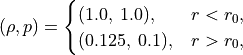
with zero initial velocity everywhere. The procedures to obtain an unsteady solution are presented as follows:
Convert mesh:
user@Computer ~/pyBaram$ pybaram import explosion.cgns explosion.pbrm
Partition the mesh:
user@Computer ~/pyBaram$ pybaram partition <ranks> explosion.pbrm explosion_p.pbrm
Run the parallel simulation:
user@Computer ~/pyBaram$ mpirun -n <ranks> pybaram run explosion_p.pbrm explosion.ini
Convert the solution to a VTK file for visualization:
user@Computer ~/pyBaram$ pybaram export explosion_p.pbrm out-0.25.pbrs out.vtu
After visualizing the solution in ParaView, you should obtain the following result.
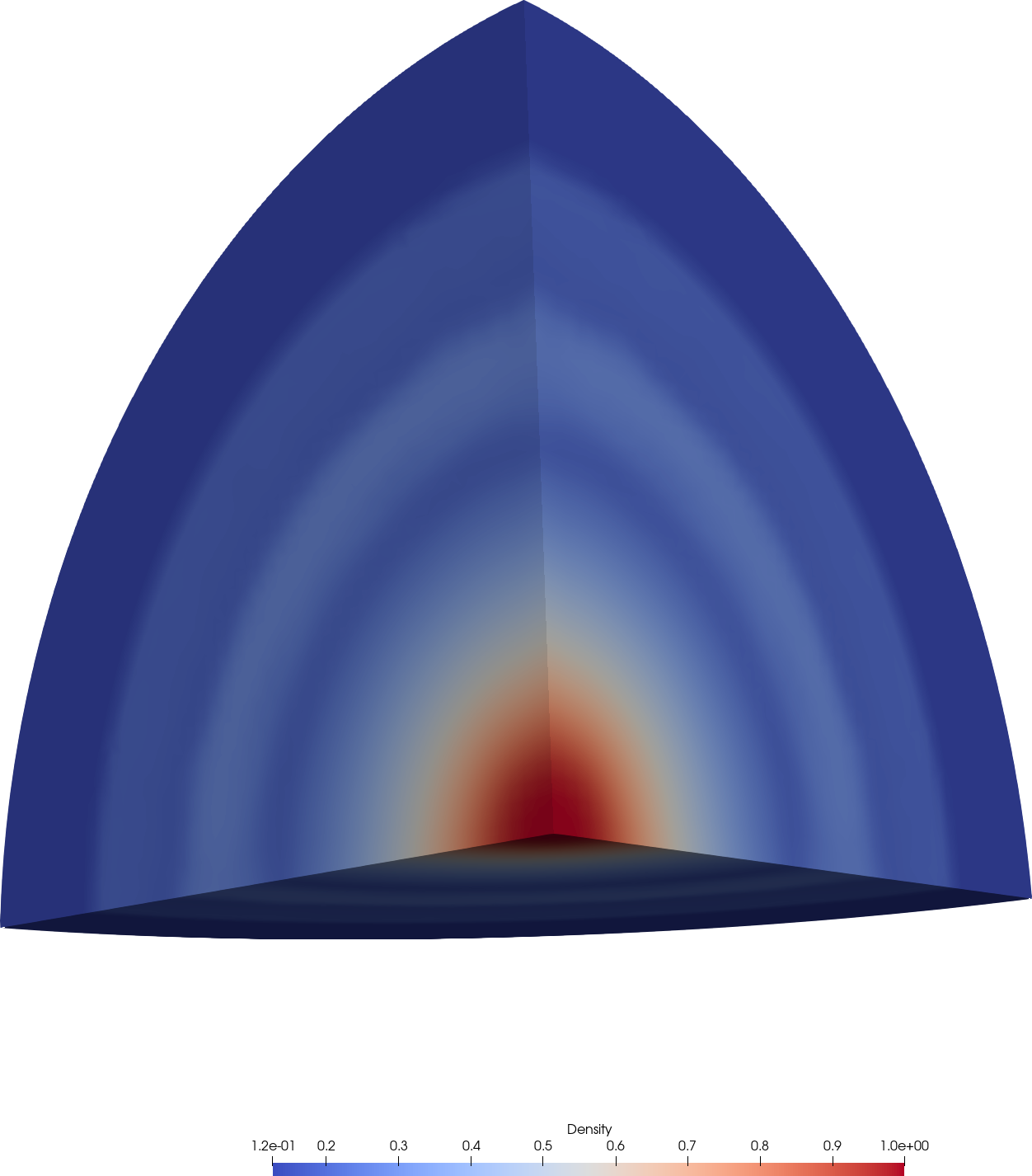
Density contour of explosion problem
Transonic flow over RAE2822 airfoil
This example considers transonic flow over the RAE2822 airfoil, which is a well-known benchmark case. The flow conditions correspond to the NPARC RAE2822 Case 4 test case, with detailed specifications available from the NPARC validation page. The computational mesh is obtained from the SU2 tutorial page.
The free-stream conditions are defined as

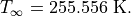
where the Reynolds number is based on the chord length  . The free-stream temperature is
A fully turbulent RANS simulation is performed under transonic conditions. The procedures to obtain a steady-state solution are presented as follows:
Convert mesh:
user@Computer ~/pyBaram$ pybaram import rae2822.cgns rae2822.pbrm
Running simulations:
user@Computer ~/pyBaram$ pybaram run rae2822.pbrm rae2822.ini
Convert the solution to a VTK file for visualization:
user@Computer ~/pyBaram$ pybaram export rae2822.pbrm out-10000.pbrs out.vtu
After visualizing the solution in ParaView, you should obtain the following result.
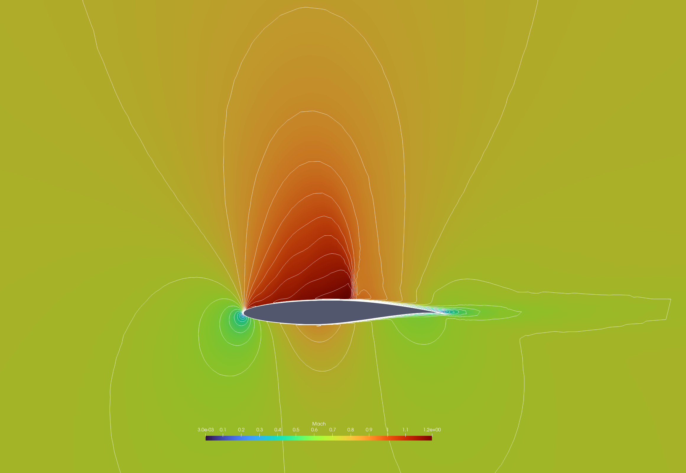
Mach contour of flow over RAE2822 airfoil
Transonic flow over ONERA M6 wing
This example considers transonic flow over the ONERA M6 wing, which is a standard benchmark for three-dimensional transonic flow simulations. The flow conditions follow the ONERA M6 test case documented in the NASA Turbulence Modeling Resource.
The free-stream conditions are defined as

where the Reynolds number is based on the root chord length. The free-stream temperature is

A fully turbulent RANS simulation is performed under transonic conditions. The procedures to obtain a steady-state solution are presented as follows:
Convert mesh:
user@Computer ~/pyBaram$ pybaram import oneram6.cgns oneram6.pbrm
Partition the mesh:
user@Computer ~/pyBaram$ pybaram partition <ranks> oneram6.pbrm oneram6_p.pbrm
Run the parallel simulation:
user@Computer ~/pyBaram$ mpirun -n <ranks> pybaram run oneram6_p.pbrm oneram6.ini
Convert the solution to a VTK file for visualization:
user@Computer ~/pyBaram$ pybaram export oneram6_p.pbrm out-3000.pbrs out.vtu
After visualizing the solution in ParaView, you should obtain the following result.
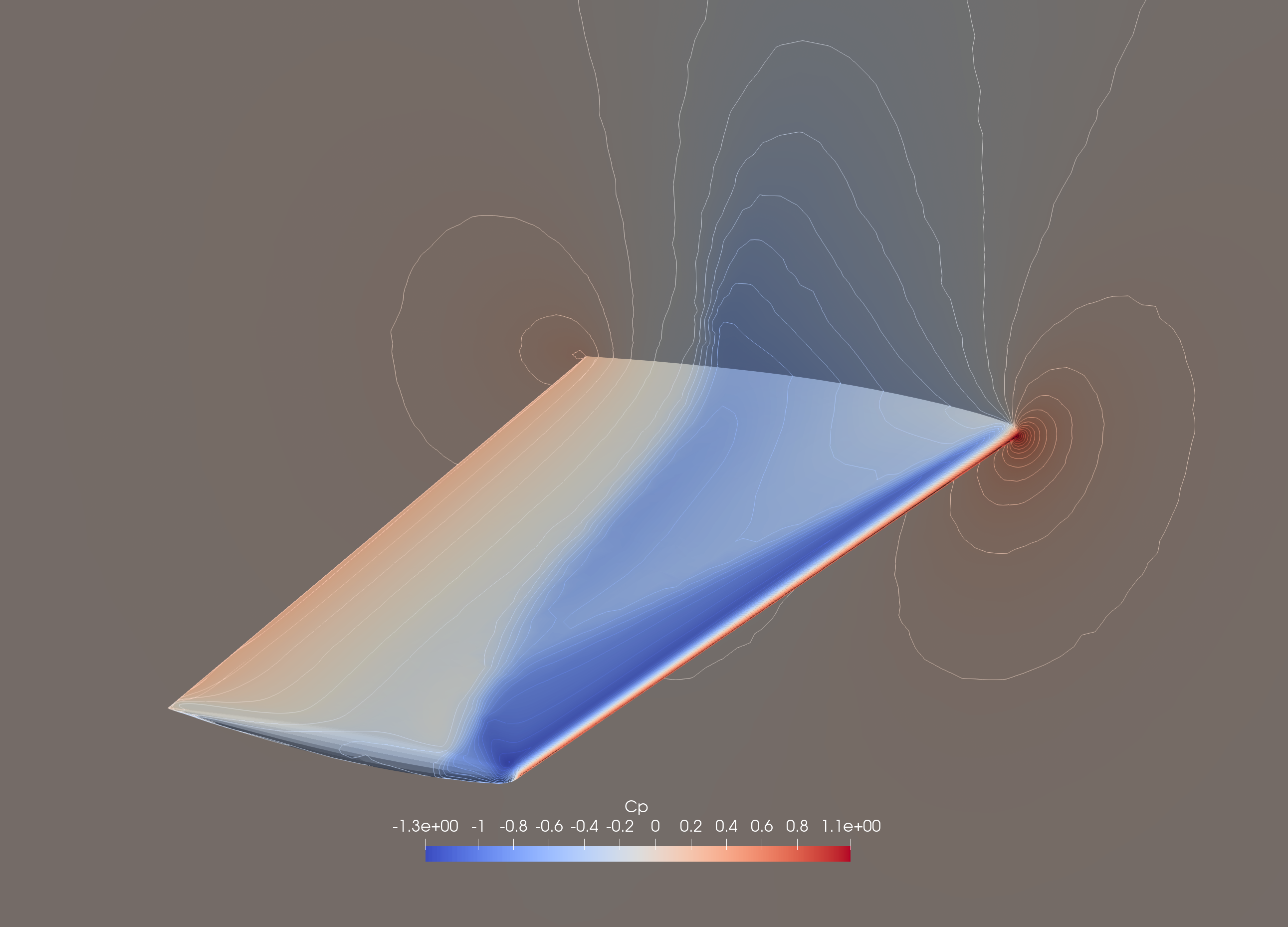
Pressure contour of ONERA M6 wing surface
Supersonic flow over HB-2 model
The HB-2 model is a standard test case for an axisymmetric body. Detailed flow conditions and experimental data are available in the AEDC technical report.
The free-stream conditions are defined as

where the Reynolds number is based on the body diameter  .
.
A fully turbulent RANS simulation is performed under supersonic conditions. The procedures to obtain a steady-state solution are presented as follows:
Convert mesh:
user@Computer ~/pyBaram$ pybaram import hb2.cgns hb2.pbrm
Partition the mesh:
user@Computer ~/pyBaram$ pybaram partition <ranks> hb2.pbrm hb2_p.pbrm
Run the parallel simulation:
user@Computer ~/pyBaram$ mpirun -n <ranks> pybaram run hb2_p.pbrm hb2.ini
Convert the solution to a VTK file for visualization:
user@Computer ~/pyBaram$ pybaram export hb2_p.pbrm out-5000.pbrs out.vtu
After visualizing the solution in ParaView, you should obtain the following result.
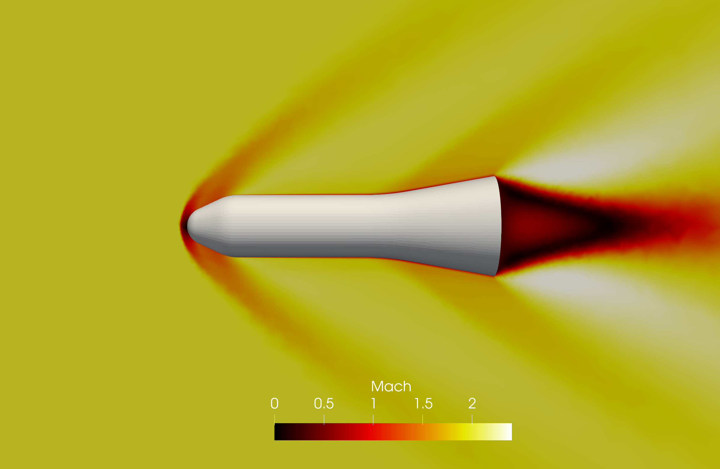
Mach contour around HB-2 model at  .
.